
Production Cost Model
Modo's tool for making power price projections
System model
The following describes a generalized version of our power market modeling framework. While the core structure and methodology are consistent across regions, specific implementations — including market rules, input data and operational constraints — vary by geography. Detailed region-specific assumptions and inputs are documented separately.
The table below outlines key features of our system model across different regions. It provides a high-level comparison of modeling scope and structure by market.
| Feature | ERCOT | Europe | GB | CAISO (WIP) |
|---|---|---|---|---|
| Production Cost Model | Yes | Yes | Yes | Yes |
| Geographic Granularity | Nodal ~5500 nodes | Hybrid | Zonal | Nodal |
| Time Granularity | Hourly | Hourly | 30m | 30m |
| Power Flow Modeling | Linearized OPF | Linearized OPF | N/A | Linearized OPF |
| Capacity Expansion | Coming soon | Coming soon | Coming soon | Coming soon |
Production cost modelling
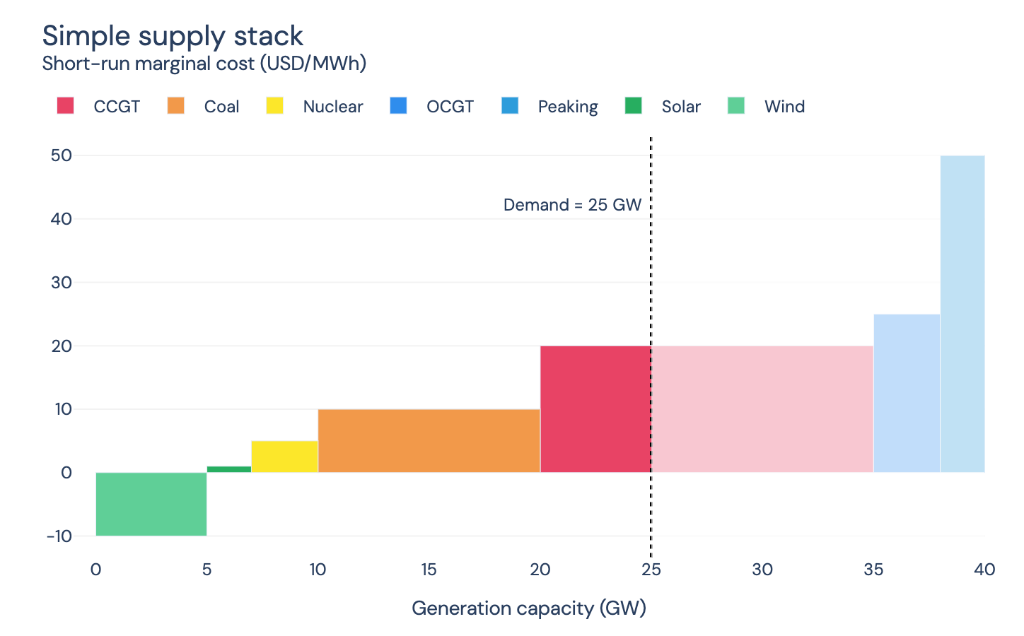
The production-cost model is a key component of Modo's forecasting tool and simulates the optimal behavior of a power system. Specifically, it decides how to dispatch generation across various technology types to ensure supply meets demand at the lowest system cost, all while respecting the limits of the transmission network.
Generators
The model includes a full fleet of generators, representing all major fuel and technology types e.g. natural gas (combined cycle, single cycle, reciproacting engines), coal, nuclear, hydro, wind, solar, etc. Each generator is modeled with technical and economic constraints that govern its behavior, such as ramp rates, and efficiency, start costs and running costs.
Outages
Outages are captured using historical patterns to reflect both planned and unplanned events. Each generator is assigned availability profiles based on observed outage rates by technology type and region. This approach ensures that generator availability reflects realistic operating conditions.
Variable Renewable Generation (Wind and Solar)
Wind and solar generation is modeled with region‑specific “weather years,” each tying capacity‑factor profiles to a particular historical year derived from meteorological data and actual generation, capturing spatial and temporal variability.
Key elements include:
- Hourly capacity factors based on multi-year historical weather and generation data.
- Regional granularity, with profiles aligned to renewable resource zones.
This modeling ensures that the variability and intermittency of renewables are realistically reflected in system dispatch and pricing outcomes.
Costs
Generator dispatch is driven by a combination of short-run marginal costs (SRMC) and start-up costs, both of which are modeled explicitly. Both cost components are technology-specific and calibrated using publicly available and proprietary datasets where available.
SRMC represents the cost of producing one additional unit of electricity while the unit is already online, and it forms the basis for economic dispatch within the model.
- SRMC includes the variable operating costs incurred during normal operation:
- Fuel costs (based on heat rates and fuel prices)
- Variable operations and maintenance (VOM) costs
- Carbon costs (where applicable)
Start-up costs influence unit commitment decisions, ensuring that peaking plants or inflexible units are only brought online when economically justified by the system conditions.
- Start-up costs capture the additional cost associated with bringing a generator online from an offline state:
- Fuel required for start-up
- Wear-and-tear or fixed O&M charges incurred on start
The model incorporates bid steps for all generators to reflect observed bidding behavior during periods of system scarcity or high load. These steps allow for mark-ups above SRMC, capturing price formation dynamics under tight conditions and better representing real-world market outcomes.
Storage
Grid-scale batteries, are modeled as bi-directional assets with both charging and discharging capabilities. The model tracks state of charge (SoC), round-trip efficiency, and power/energy limits.
Key constraints include:
- Maximum charge/discharge rates
- Energy capacity
- Minimum/maximum state of charge
- Round-trip efficiency losses
Storage is dispatched economically to maximize system cost savings or arbitrage opportunities.
Load
Load is represented at a high temporal and spatial resolution, aligned with historical or forecast demand profiles. It can be broken down by sector where applicable (e.g., residential, commercial, industrial) and may include demand-side flexibility or response behavior if supported by the region's data.
Features:
- Hourly (or finer) demand profiles
- Regional distribution of load
- Flexible load blocks
Transmission
Zonal Modeling
All market models incorporate fundamental zonal transmission constraints and elements, including:
- Transfer capacity limits on zonal interties
- Thermal limits and directional flow constraints
- Wheeling charges or congestion pricing mechanisms aligned with regional market designs
Power Flow Modeling
In certain regions, detailed power flow modeling is employed because grid physics significantly impact pricing and dispatch decisions. For these markets, the model integrates a linearized DC optimal power flow (OPF) formulation, explicitly capturing these operational constraints.
Power flows are calculated by solving for voltage phase angles at each node, with flows along transmission lines governed by their reactance and constrained by thermal transfer limits. The model ensures that all flows respect physical constraints while minimizing total system dispatch cost.
Transmission Interfaces
To represent regional flow constraints and system bottlenecks, the model incorporates transmission interfaces — predefined boundaries or paths across which aggregate flows are tracked and limited that critical network paths defined by the system operator. These interfaces are tailored to the structure and operational conventions of each market.
Each interface includes:
- Thermal transfer limits, typically aligned with system-operator-defined constraints
- Directional flow considerations, where applicable
Interfaces provide an additional layer of constraints to reflect more systemic transmission congestion and regional price separation.
Assumptions and caveats
- Linearized physics: Power flows follow DC approximations — flows are linear functions of phase angle differences and line reactances.
- No losses: Line losses are not explicitly modeled under the DC approximation.
- No contingencies: The model represents a base-case scenario without simulating N-1 security constraints or transmission outages.
Power Balance
At each location and time step, the model enforces a power balance constraint: total supply (generation, storage discharge, and imports) must equal total demand (load and storage charging). This constraint ensures physical feasibility and underpins the calculation of marginal prices across the system.
To maintain system feasibility under all conditions, the model includes a loss-of-load resource, often referred to as a "generator of last resort." This resource has a very high cost and is only dispatched when no other generation or flexibility is available. It acts as a backstop to represent involuntary load shedding and ensures the optimization always has a feasible solution.
The shadow price of the power balance constraint at each location and time represents the marginal cost of meeting one additional unit of demand, forming the basis of modeled energy prices.
Outputs
Zonal Model
- Plant level behaviour
- The generation output and run hours of each plant at every point in time
- Generator start-up and shut-down
- Economic curtailment of renewables
- Storage behaviour including charge, discharge, state of charge and cycling
- Transmission
- Flows along all transmission lines
- Congestion rents
- The price of energy - calculated as the cost of producing an additional unit of electricity at each region in the model (aka the shadow price of the power balance constraint).
Optimal power flow model (if applicable)
- Nodal locational marginal prices (LMP) at every node — representing the marginal cost of serving one additional unit of demand at that location, and considering both generation costs and network congestion.
- Congestion rents, derived from price differences across constrained lines
- Line-level power flows, including directionality and constraint binding status
Capacity expansion (WIP)
Capacity expansion modeling is under development and will allow the simulation of long-term investment decisions in generation and storage assets. It will enable the model to optimize future capacity additions based on projected system needs, costs, and policy goals.
This feature is being designed to integrate seamlessly with the production cost model and will support scenario analysis for planning and policy evaluation.
Battery dispatch model
The battery dispatch model is a key component of our power market modeling framework, designed to optimize battery storage operations across energy and ancillary services markets. The model determines the optimal charging and discharging schedule for grid-scale batteries while respecting technical constraints and market rules.
Key Features
Physical Characteristics
- Power Rating: Separate import (charging) and export (discharging) power limits
- Energy Capacity: Defined by power rating and duration (hours)
- Efficiency: Defaults to 88% round-trip efficiency
- State of Charge (SoC): Tracks energy level with minimum and maximum bounds
Market Participation
The model optimizes battery operations across multiple markets:
-
Energy Market
- Real-time market participation
- Price arbitrage between charging and discharging periods
- Bid steps to reflect scarcity pricing
-
Ancillary Services
- Regulation Up/Down
- Responsive Reserve Service (RRS)
- Non-Spinning Reserve
- Emergency Response Service (ECRS)
-
DA-RT Energy Arbitrage
- Not yet implemented
Operational Constraints
Cycling Limits
- Daily Cycling: Maximum number of full charge-discharge cycles per day
- Annual Cycling: Optional annual cycling budget that dynamically adjusts daily limits based on price spreads
- Cycle Charge: Cost per cycle to account for degradation ($/MWh)
State of Charge Requirements
- Headroom: Minimum energy reserve required for downward regulation
- Footroom: Minimum energy reserve required for upward regulation
- Service-Specific Requirements: Different SoC requirements for various ancillary services
Degradation Modeling
- Tracks cumulative cycles over time
- Adjusts effective energy capacity based on degradation profile
- Optional repowering threshold to reset degradation
Optimization Framework
The model uses a mixed-integer linear programming (MILP) approach to maximize revenue while respecting all constraints:
Objective Function
Maximizes total revenue from:
- Energy market arbitrage
- Ancillary service commitments
- Less cycling costs
Key Constraints
-
Power Balance
- Charging + ancillary service imports = discharging + ancillary service exports
- Respects power rating limits
-
Energy Balance
- State of charge updates based on net energy flows
- Accounts for round-trip efficiency losses
-
Ancillary Service Requirements
- Market size limits
- Activation rates
- Sufficient headroom/footroom for service provision
-
Cycling Limits
- Daily cycle budget
- Annual cycle budget (when enabled)
Outputs
The model provides detailed operational data including:
- Hourly state of charge
- Charging/discharging schedules
- Ancillary service commitments
- Market revenues by service type
- Cycle counts and degradation tracking
Updated about 1 month ago