
Overview
An overview of the inputs, modeling and outputs, specific to the ERCOT implementation of our forecast
ERCOT
Our system-wide ERCOT simulation runs at hourly granularity across the entire modeling horizon. As such outputs such as price, generation output, transmission flows, etc are all determined at the hourly level. Our modeling horizon extends to 2050, with varying levels of locational granularity:
- Nodal modeling at the substation level from 2025 - 2034.
- Zonal modeling at load zone level (North, South, Houston, and West) for 2034 onwards.
This split reflects a trade-off between modeling detail and input data quality for distant future. In the nearer term, there is more detailed, locational data on system topology for load, generation and transmission. As such, we can appropriately capture critical locational signals — congestion, basis risk, and site-specific value drivers. Beyond 2034, there is less locational detail available and a higher level uncertainty around system topology. It is our belief, that speculating on the specifics of a 2050 topology effectively introduce 'false precision', that is a model that outputs highly detailed results that appear accurate but are actually unreliable due to the underlying uncertainty of the inputs.
To avoid this, we feel it is most appropriate to move to a zonal representation of the system for the later years in the horizon. This enables us to maintain some location-awareness in the model whilst avoiding the pitfalls of false precision.
Inputs
The table below summarizes the key input types to our model, and provides a high-level description of how each input is constructed alongside key data sources used to inform our assumptions. Further details for each of these inputs can be found at the links provided.
| Input Type | Input | Summary | Key Data Sets |
|---|---|---|---|
| Generation | Capacity buildout | Capacity additions up to 2031 are informed by ERCOT’s GIS queue, filtered by project maturity. Beyond 2031, a stylized buildout approach maintains system adequacy, guided by external projections like EIA’s AEO. | ERCOT GIS Queue, EIA Generator Inventory, EIA Annual Energy Outlook |
| Generation | Renewable load factors and outages | Renewable resource availability and outage profiles are empirically modeled using historical SCED High Sustained Limit (HSL) data to capture seasonal and hourly variability. | ERCOT SCED High Sustained Limit (HSL) data |
| Generation | Start costs | Start costs for thermal technologies are determined empirically based on historical SCED data and forecast fuel prices. | ERCOT SCED Data, EIA AEO commodity price forecasts |
| Generation | Short-run marginal costs | Short-run marginal costs (SRMCs) are empirically estimated for each generation site using historical SCED pricing data combined with forward-looking fuel commodity price forecasts. | ERCOT SCED Data, EIA AEO commodity price forecasts |
| Demand | Nodal Demand | Nodal demand is modeled hourly at the substation level through 2034, combining weather zone load shapes and nodal distribution factors. Beyond 2034, stylized zonal growth assumptions extend demand projections to 2050. | ERCOT RTP Load Profiles, ERCOT LTSA, Permian Basin Study |
| Transmission | Nodal Transmission Network | Up to 2034, the nodal transmission network is built from individual lines with detailed ratings and reactance values, updated to reflect planned topologies from ERCOT’s Regional Transmission Plan and key Permian Basin upgrades. | ERCOT RTP Economic Start Cases, CIM Ratings Report, Permian Basin Reliability Planning Study |
Modeling
Alongside the core modeling functionality described here, there are additional market features modeled in our representation of the ERCOT system.
Unit Commitment
Unit commitment refers to the modeling of generator on/off decisions through binary variables that determine whether a generating unit is online or offline at any given hour.
In the model, a binary commitment variable is assigned to each thermal generating unit. Operational limits — specifically minimum and maximum generation levels — are conditional on this commitment status. When a unit is online, it must operate within its defined minimum stable output and maximum output levels. When offline, a unit's output is constrained to zero. This structure allows the model to capture key operational behaviors such as startup costs, minimum load requirements, and restricted flexibility, reflecting real-world generator limitations.
Reserve Margin
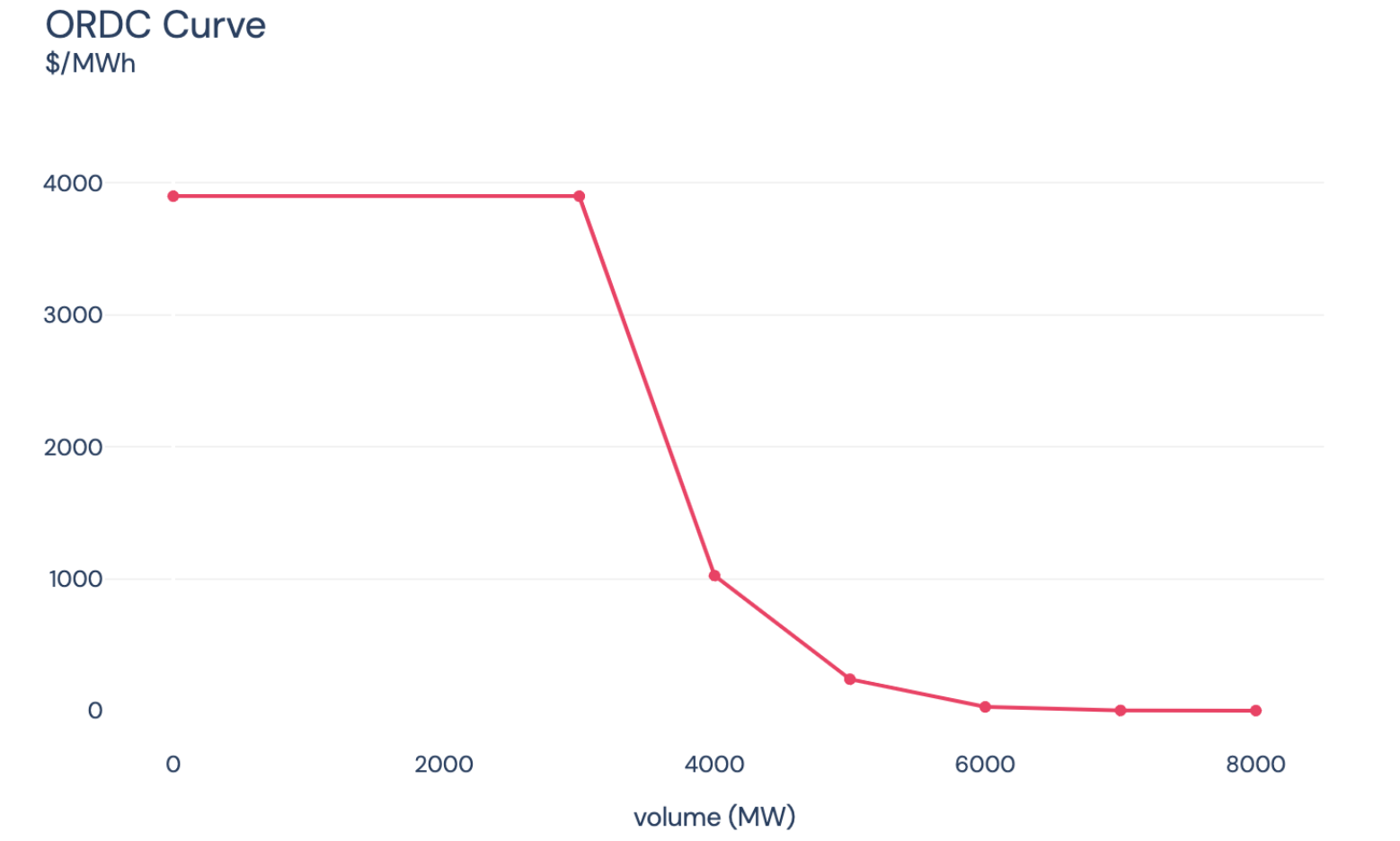
Reserve margin refers to the amount of available generation capacity above expected system demand, maintained to ensure grid reliability in the event of unexpected contingencies such as generator outages or rapid demand spikes. In ERCOT, reserve margin requirements are closely linked to the Operating Reserve Demand Curve (ORDC) structure, which incentivizes maintaining sufficient reserves through scarcity pricing mechanisms.
In the model, reserve margin is proxied by measuring available headroom across dispatchable thermal generation and energy storage assets across the whole system. Specifically, it is calculated as the sum of thermal generator headroom (High Sustained Limit minus Base Point) and available storage capacity (accounting for state of charge constraints). A fixed system-wide operating margin of 8 GW is enforced, reflecting the width of the ORDC curve and inspired by ERCOT’s Real-Time Operating Capacity (RTOLCAP) concept.
If reserves fall below 8 GW, "reserve of last resort" is used to meet the reserve required and is priced in line with ORDC. Below the Minimum Contingency Level (MCL), ORDC prices spike towards the Value of Lost Load (VoLL), creating highly punitive costs for failing to maintain sufficient reserves. This structure mirrors ERCOT’s real-time market operations and ensures that system reliability pressures are reflected in dispatch outcomes without imposing hard infeasibility constraints.
Generic transmission constraints
Generic Transmission Constraints (GTCs) are groups of transmission lines for which directional flow limits are imposed on the total flow across the interface. These constraints are designed to reflect grid stability limits and are pre-defined ahead of real-time dispatch to allow ERCOT’s SCED to maintain system reliability without requiring full stability analysis during dispatch.
GTCs are modeled by mapping ERCOT’s published definitions — which specify both the constituent lines and the flow restrictions — onto the network represented in the model. Each GTC aggregates the flow across its defined set of lines, and enforces a maximum allowable directional flow limit.
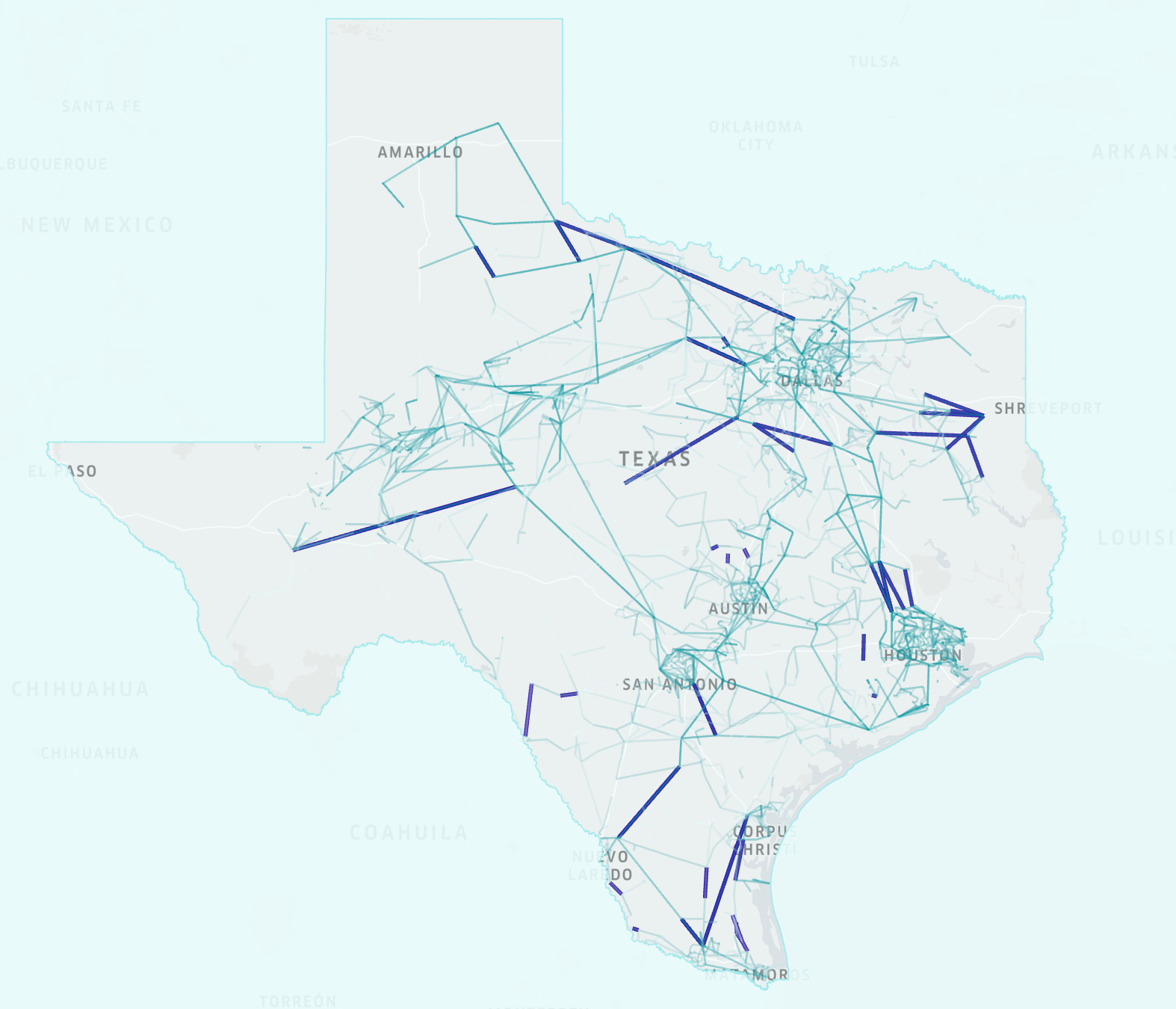
Transmission lines are displayed in light blue with GTCs highlighted in dark blue
Outputs
Macro databook
The Macro Databook summarizes key system-level outputs with yearly granularity, capturing installed generation capacity by technology type, generation volumes, commodity prices, zonal electricity prices, and top-bottom two-hour spreads (TB2s). Provided in CSV format, it represents Modo’s proprietary view on capacity expansion pathways, future commodity prices, and market dynamics, clearly reflecting the core assumptions underpinning our ERCOT modeling approach and enabling high-level market analysis.
Site specific databook
The site specific databook provides detailed monthly and annual performance metrics for individual battery assets, including cycling behavior, merchant, and ancillary service revenues. Cycling counts and prices are averaged over each period, while total revenues are also presented on a per MW basis, to facilitate asset benchmarking and investment evaluation. These revenue outputs can directly support financial modeling, due diligence processes, and investment decisions.
FAQs
General
How often do you update the model?
We update the model on a quarterly basis, incorporating the latest data, market developments, and structural changes. Each update may also include improvements to model features or functionality, reflecting our ongoing development priorities.
Can we use the forecast to support BESS financing?
Yes — the forecast is structured to support investment cases and includes merchant and ancillary revenues across multiple scenarios. Outputs are designed to be suitable for use in financial models, investor decks, or due diligence processes.
Fundamentals Model
How do you model storage cannibalization and market saturation?
The model captures price suppression effects through endogenous storage behavior. As more storage enters the system, competition for arbitrage and ancillary services naturally leads to diminishing returns.
How do you model scarcity pricing in ERCOT?
Scarcity pricing is modeled explicitly using a simplifcation of ERCOT's ORDC (Operating Reserve Demand Curve) mechanism. When reserves are tight, prices rise in line with the published ERCOT ORDC parameters, reflecting real-world scarcity pricing behavior.
How do you model negative prices?
Negative prices arise naturally in the model when supply outstrips demand — typically during high wind or solar output and low load conditions. We also factor in Production Tax Credits (PTCs) for eligible wind and solar assets by embedding them into the SRMC, which can push bids below zero. This reflects real market behavior, where PTC-backed projects are willing to generate through negative pricing events. While PTCs are phasing out for new builds, many ERCOT assets still qualify, making this a persistent feature in the near term.
Can the model simulate curtailment?
Yes — curtailment is captured when transmission constraints or system-wide oversupply prevent full renewable dispatch. The model reflects both economic curtailment and curtailment due to network constraints.
How do you model ancillary services and real-time co-optimization?
We don’t model ancillary services as separate markets within the system-wide model; Instead, we proxy reserve provision by holding back capacity in line with system reserve margins — capturing the key trade-off between energy and reserve availability. Ancillary service prices themselves are modeled using a regression model trained on historical ERCOT data. It links energy prices to observed ancillary service prices across Reg-Up, Reg-Down, RRS, and NSRS. This lets us forecast service prices based on energy price outputs from the fundamentals model.
Dispatch Model
How do you model and validate storage revenues?
Storage revenues are modeled using a detailed dispatch engine that optimizes battery behavior across energy and ancillary markets. To ensure realism, we calibrate the model using the Modo benchmark — a proprietary dataset of historical storage revenues in ERCOT.
This calibration process adjusts model parameters (e.g. efficiencies, cycling limits, market participation assumptions) to align modeled outcomes with real-world operator behavior. By grounding the forecast in observed revenue profiles, we can better capture how storage assets actually perform — not just in theory, but in practice.
Updated about 1 month ago